

Propagação de ondas de choque em experimentos de tubos de choque


Computational Fluid Dynamic Simulation of a Non-reactive Propagating Shock Wave in a Shock Tube
Leonel Rincon Cancino, Dr. Eng.
Amir Antônio Martins Oliveira, Ph.D.
Combustion and Thermal Systems Engineering Laboratory – LABCET
Mechanical Engineering Department
Federal University of Santa Catarina
Brazil.
Mustapha Fikri, Dr.
Christof Schulz, Dr.
Institute for Combustion and Gasdynamics – IVG
University of Duisburg-Essen
Germany
Contact: Prof. L.R.Cancino – leonel@labcet.ufsc.br
Abstract: The study of ignition delay for practical fuels in the low to intermediate temperature range (700 to 1100 K) in shock tube requires test times of the order of milliseconds. The test time available in practical devices is however limited by the arrival of the contact surface and the conditions in the igniting mixture are affected by the growth of boundary layers. In this paper, we simulate the non-reactive shock wave propagation by computational fluid dynamic as a tool to aid understanding the in°uence on boundary layer effects. The simulation is applied to the high pressure shock tube of IVG at the University of Duisburg-Essen. The prediction of shock speed, pressure and temperature are compared to measurements and to the output of CHEMKIN’s SHOCK package.
1. Introduction
The shock tube facility is extensively used for studying unsteady short-duration phenomena in the fields of aerodynamics, physics and chemistry. A shock tube consists of a long tubular reactor which is separated by a thin diaphragm into two sections. One of them, the low-pressure section, is filled with the test gas. The compressed driver gas is fed into the second part, the high-pressure section. In the operation of shock tubes, at time t = 0 s, Figure 1(a), the diaphragm bursts and a series of compression waves rapidly collapses into a normal shock wave. The wave propagates at supersonic speed in the driven section and sets the fluid behind it in motion in the direction of the shock with the velocity u_iw, as in Figure 1(b) and (c). Behind the incident wave, the contact surface between the driven and driver gases is moving with the velocity u_cs. The difference between u_iw and u_cs permits that the test gas achieves the condition of high pressure and temperature (T5, p5) behind the reflected wave before the contact surface displaces the uniform conditions. This is represented in Figure 1(d) and (e). Simultaneously, within the driver section, a set of rarefaction waves propagate in an opposing direction inside the driver gas. The arrival of the rarefaction waves also disturbs the sample gas. The time interval between the arrival of the reflected wave and of the contact surface is the available time for measurements Δt (ms), represented in Figure 1(f). When conditions on both sides of the contact surface are chosen appropriately, the interaction of the reflected wave with the contact surface does not generate additional waves and the contact surface is also brought to rest. This is called the tailoring of the driver gas. Successive time-pressure distributions indicating the shock front position can be plotted in an x-t diagram, giving the typical distance-time diagram, as shown in Figure 1(f), and commonly found in the literature (Saad (1993), Zel’dovich et al. (1966), Kee et al. (2000)). The conditions behind a shock wave are well predicted by one-dimensional models, Bird et al. (1954). When diffusion effects are neglected, the shock wave manifests itself in the solution of the conservation equations as a mathematical discontinuity, as represented in Figure 1.
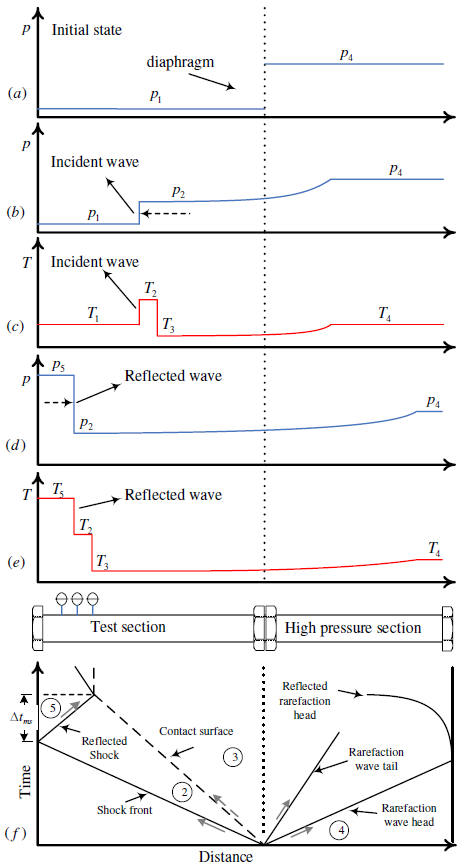
Figure 1. Operation of a shock tube (Adapted from Zel’dovich et al. (1966)) and Distance-time diagram in shock tube (Adapted from Kee et al. (2000))
These models formulated in steay-state are used in the SHOCK program of the CHEMKIN package. When dissipative processes are taken into account, on the other hand, the shock wave structure changes, the contact surface spreads out into a contact region and boundary effects appear at the tube wall. The net effect of disspative effects on the shock wave structure is to change the discontinuity into a slightly gradual transition which takes place within a distance of a few molecular mean free paths l_0 (Bird et al. (1954), Zel’dovich et al. (1966b)). Typical values of shock thickness are 1.0 to 4.0 molecular mean free paths for l_0 of the order of 1×10⁻⁵ cm. Since the gas undergoes a considerable change of properties in such a small distance, the Navier-Stokes equation is often insuffciently accurate to describe the structure and thickness of the wave (Bird et al. (1954), Zel’dovich et al. (1966b)). Dissipative effects also manifest at interfaces, including the contact surface and the walls, through the formation and growth of boundary layers. In an ideal shock-tube experiment both the shock and the contact surface are plane sharp discontinuity surfaces, moving with constant velocity, and the flow in between is uniform. The presence of a wall boundary layer causes the shock to decelerate (shock attenuation), the contact surface to accelerate, and the flow to be non-uniform.
Figure 2 (adapted from Mirels (1963)), presents a rendering of (a) the x-t diagram and (b) the flow velocity profiles at time ta for an incident shock wave. The difference between the ideal and the real positions of the shock and the contact surface can be noticed. Mirels (1963) also provide a relation for the critical Reynolds number for transition from laminar to turbulent regime in the boundary layer for low pressure shock tubes. He shows that transition to turbulent boundary layer becomes more likely as the initial pressure of the shock tube and the shock Mach number increase. Rudinger (1961) reported the effect of the boundary layer growth on shock reflection from a closed end. He showed that the pressure behind a propagating shock wave increases slightly with time as a result of the growing of the boundary layer.
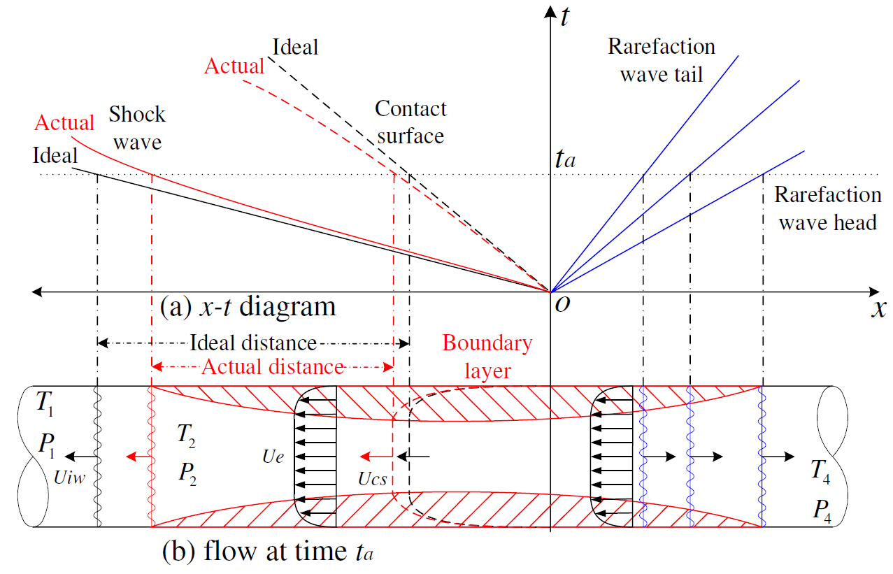
Figure 2. Boundary layer in shock tube (Adapted from Mirels (1963))
Even though the structure within a shock wave may not be captured accurately by a formulation based on continuum conservation equations (continuity, Navier-Stokes, mass of chemical species and energy), it is possible that they provide an estimate of general trends of shock wave propagation, such as front speed, pressure and temperature increase. Most important, continuum models should be able to capture interface phenomena, such as movement and spread of contact surface and wall boundary layers. For this, the model has to take into account the possibility of transition to turbulence. Therefore, the effect of boundary layer growth on the magnitude of the pressure increase at the measurement region (at the end of the shock tube) as well as the arrival of the contact surface, defining the measurement window, can be estimated using numerical simulation. Recent reviews discuss the state of the art in numerical modeling of shock wave and turbulent boundary layer interaction, Knight et al. (2003), Mundt et al. (2007), Edwards (2008). Knight et al. (2003) present results from RANS, DNS and LES simulations of a 2-D shock impingement, among other test problems. They show that RANS models are able to reasonably predict the surface pressure distribution, but there are significant differences among predictions of different RANS models of velocity distribution, surface skin friction and heat transfer. In their review, the κ-ω, κ-ε and the Baldwin-Lomax-Panaras models were more successful. There are not many works available on simulation of shock tube. From the more recent work, Tsuchida et al. (2006) performed direct numerical simulation of the shock tube used by Sod (1978), in order to confirm the applicability of their compressible CFD scheme with node-by-node finite elements. The density results of the simulations were then compared to theoretical results and good agreement was found. Al-Falahi et al. (2007) used CFD to evaluate the performance of the Short-Duration Hypersonic Test Facility at Universiti Tenaga Nasional, Selangor Darul Ehsan, Malaysia. They analyzed the parameters that affected the performance of the device using both experiments and simulation using RANS (Reynolds-Averaged Navier-Stokes) models. As a major result, they found that He/CO2 was the best combination driver/driven gases to obtain high Mach numbers. Also, in their work the predicted shock wave strength using CFD was always higher compared to the measurements.
Here, a numerical model based on a continuum compressible flow formulation is applied to the conditions prevailing in the shock tube of the IVG at University of Duisburg-Essen during a typical high pressure, low temperature, ignition delay test for a stoichiometric ethanol-air mixture. The model is applied to a 2D-axisymmetric geometry and neglects chemical reactions. Four models are tested. One, uses the conservation equations for mass, mass of chemical species, momentum and energy, without the use of a turbulence model. The other three use RANS equations employing three turbulence models, the standard κ-ε model, the standard κ-ω model and the Reynolds Stress Model – RSM. The predictions are then compared to measurements of shock wave speed and to the conditions behind incident and reflected shock waves predicted by the 1D code SHOCK of the CHEMKIN package. Finally limitations of the shock tube experiments are discussed and directions for future work are pointed-out.
2. Experimental setup
Experiments were carried out in the high-pressure shock tube at IVG, Duisburg-Essen University, Duisburg, Germany, in order to validate the numerical results. The shock tube, presented schematically in Figure 3, has an internal diameter of 90 mm. It is separated by an aluminum diaphragm into a driver section of 6.1 m and a driven section of 6.4 m in length. This device was used recently to study the ignition delay time of ethanol-air mixture, Cancino et al. (2009). Before a typical experiment, the driven section was pumped down to pressures below 1×10⁻² mbar. Then, the gas mixture was prepared by injection of liquid ethanol and subsequent complete evaporation in the driven section. The total amount of ethanol and air was controlled manometrically in order to ensure the desired equivalence ratio. The shock tube was heated to 50 °C. The shock speed was measured over two intervals using three piezoelectric pressure gauges. The data were recorded with a time resolution of 0.1 μs. The temperature and pressure behind the incident and reflected shock waves, (p2, T2, p5 and T5), were computed from the measured incident shock speed and the speed attenuation using a one-dimensional shock-tube model (shock-tube code of the CHEMKIN package, Kee et al. (2000)). The experiment was carried out with synthetic air containing 79.5% N2 and 20.5% O2. The driver gas was mixed in-situ by using two high-pressure massflow controllers (Bronkhorst Hi-Tec flow meter F-136AI-FZD-55-V and F-123MI-FZD-55-V). Helium was used as the main component and Argon was added to match the acoustic impedance of the test gas. Concentrations of 5 to 20% Ar in He were required to tailor the desired shock waves. The experimental conditions are summarized in Table 1.
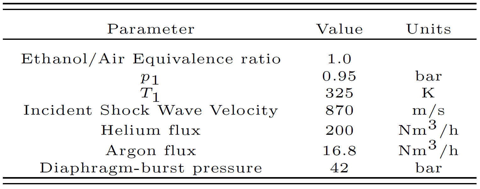
Table 1. Experimental conditions
3. Numerical simulation
The simulation model solves the transient form of the energy, species, momentum and turbulence equations in a 2D-axisymmetric geometry neglecting chemical reactions. The parameters listed in Table 1 were taken as input parameters, except the incident shock wave speed that was used as a validation parameter. All internal surfaces were assumed adiabatic. Full multi-component diffusion (using Maxwell-Stefan equations) was considered in the species transport. The simulation was performed with the commercial CFD code FLUENT 6.3.
3.1. Turbulence models
Simulations were performed using three RANS models, the standard k-e model, as proposed by Launder and Spalding (1972), the standard k-w model, proposed by Wilcox (1998), and the Reynolds Stress Model – RSM proposed by Gibson and Launder (1978), Launder (1989) and Launder et al. (1975). All turbulence models are fully implemented in the FLUENT commercial code and described in Fluent 6.3 (2006). In the two-equation RANS models, the Reynolds stresses, avg( u’_i u’_j u’_k ), resulting in the mean flow equations, are determined by modeling. In the κ-ε model, two transport conservation equations are proposed and solved for two turbulence quantities; the turbulent kinetic energy, κ, and its dissipation, ε. In this model, the flow regime is assumed completely turbulent. In the κ-ω model, equations for the turbulent kinetic energy, κ, and for the specific dissipation rate, ω are solved. In the Reynolds Stress Model, transport equations are solved for the individual Reynolds stresses, avg( u’_i u’_j u’_k ), for the dissipation w, or for other variables that provided a length or time scale for the turbulence, Pope (2000). In this way, the turbulent viscosity hypothesis is not needed, which is a great advantage over the κ-ε and κ-ω models. Accordingly, the number of conservation equations increases making the computational solution more time-expensive.
3.2. Grid independence and numerical solution
Taking advantage of the shock tube geometry, a 2D axially-symmetric computational domain was generated using the GAMBIT 2.2.30 mesh generator as described in Fluent 6.3 (2006). The computational domain has a radius of 45 and length of 12,500 mm. Figure 3 shows the computational domain.
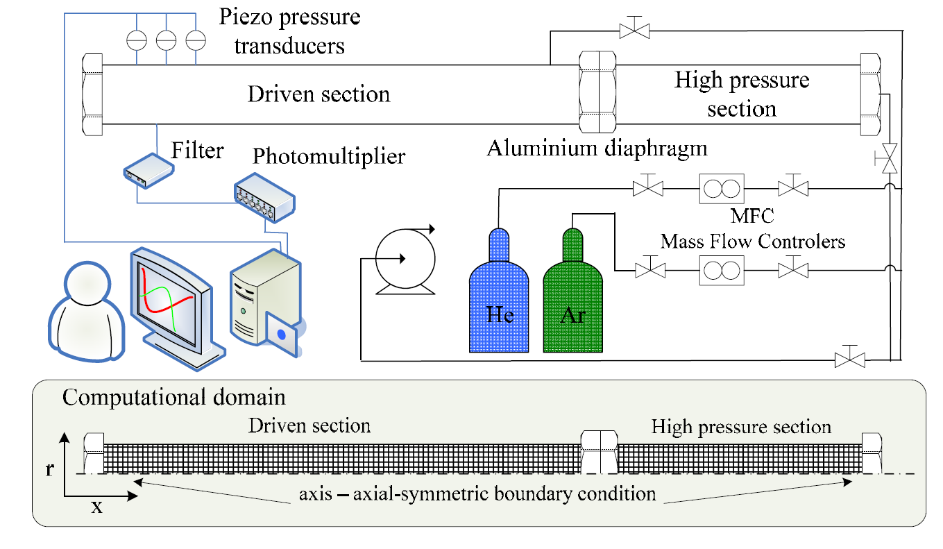
Figure 3. High pressure shock tube and computational domain
Different grids were tested and the one that provided the best trade off between having realistic and permissible computational times and having reasonable agreement with the measured values was selected. Table 2 presents the prediction of shock wave speed obtained using a coarser grid and a finer grid with twice the number of mesh points. Both grids had a refinement at the wall. We note an improvement in the prediction of shock wave speed for the finer grid, presenting a deviation in respect to the measurement of 1%. This grid was selected for the computations presented below. It had a uniform mesh with 2,325,000 nodes with resolution of 0.5 by 0.5 mm in the bulk. Near the wall a boundary layer mesh refinement was applied using four rows with a total depth of 0.053 mm and a growth factor of 1.2. The time discretization was fixed to 1×10^(-5) s.
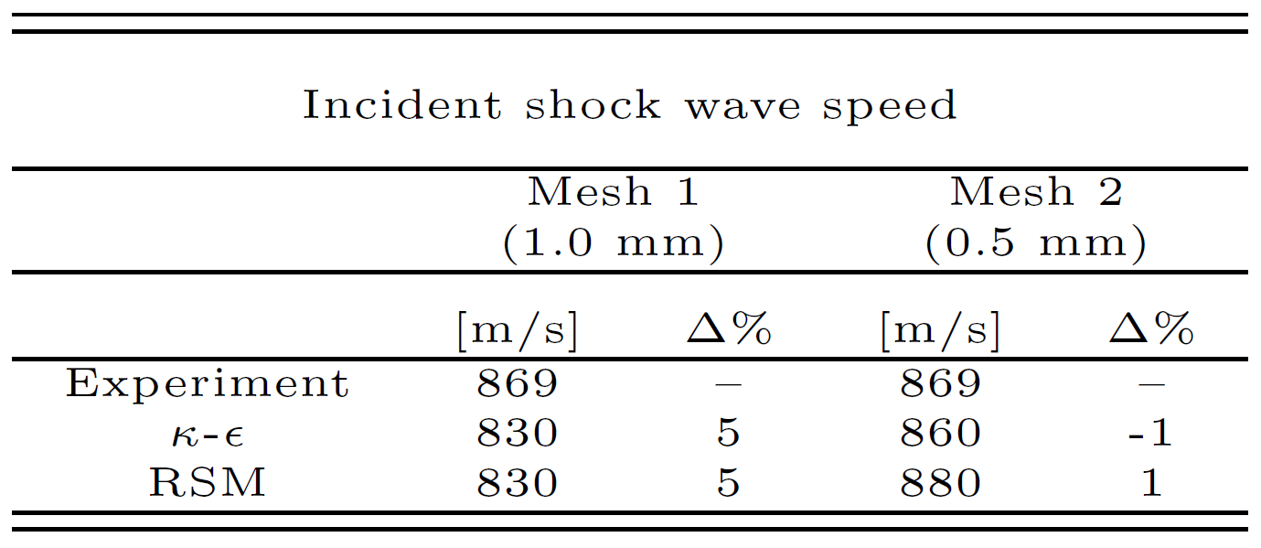
Table 2. Grid independence study
The mean simulation time, per shock simulation, using this mesh resolution was about 35 days in parallel processing using 2 PC computers Intel Core 2 Duo, 1.86 GHz, 4 GB of RAM and 2 TB memory. Note that taking a mesh resolution near the molecular mean free path, l_0, would require a total of 5.6×10^13 nodes, about 25 million times the number of nodes adopted in this work.
4. Results and discussion
We take the measured value of incident shock wave speed as the main parameter for validation. Other parameters estimated using the one-dimensional SHOCK code of CHEMKIN Kee et al. (2000) are also compared. The SHOCK program, Kee et al. (2000), uses the conditions measured before the incident shock (state 1) to calculate the conditions behind the incident shock (state 2) and behind the reflected shock (state 5) by using one-dimensional relations for the shock-wave propagation. The values are summarized in Table 3.
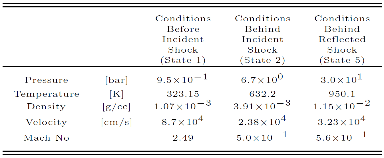
Table 3. Results of the 1D calculation from SHOCK
4.1. Prediction of wave speed
Figure 4 shows the position of the incident and reflected shock waves, the rarefaction wave and the contact surface as a function of time predicted from the simulations. In all simulations, the shock position is taken as the position along the tube axis where the pressure increases. The contact surface is taken as the position along the tube axis where the ethanol mass concentration reaches ~98% of its initial value. All the turbulence models that were applied resulted in approximately the same qualitative behavior. The position of the incident shock wave is about the same for all models except for the κ-ω which lags behind. We note that the contact surface remains approximately stationary after interacting with the reflected shock for the RSM and the κ-ω models and receeds with time for the κ-ε.
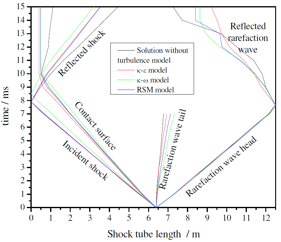
Figure 4. Distance-time diagram obtained from CFD
simulations
The useful measurement time for chemical kinetic studies, the time after the passage of the reflected wave and before the arrival of the contact surface, even with poor tailoring would be estimated in, at least, ~1.5 ms. For the reflected shock wave, the simulation without turbulence model predicts higher speeds when compared to the RANS models. The rarefaction wave is predicted with approximately the same wave speed for all models used. For the reflected rarefaction wave there is a dispersion of the wave speed results. The rarefaction wave tail is predicted with different speeds depending on the model used. Table 4 compares the numerically predicted and measured incident and the numerically predicted and calculated by CHEMKIN reflected shock-wave speeds.
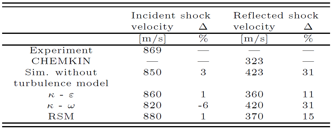
Table 4. Incident and reflected wave velocities
All models predict well the incident wave, but all over predict the reflected wave speed with also a larger dispersion. We note that a value 6% smaller of wave speed was predicted by the κ-ω model. Such a deviation of 6% in relation to the experimental value of incident shock wave seems to be small. However, using the SHOCK code, such small difference implies in differences up to 17% and 8% in the prediction for pressure and temperature behind the reflected shock wave. This would have a strong effect in the measurement of chemical kinetics. The larger deviations observed in the prediction of reflected wave speed indicate the strong effect of the choice of model in predicting the reflection of the wave at the end wall. This is due to the diffculty in predicting the dissipation and flow reversal in the proximity of the end wall as well as in predicting the complicated and unsteady shock wave pattern formed after interaction with the end wall. Since all simulations represent qualitatively the same behavior, only the RSM and the κ-ε turbulence models will be used to explore further details.
4.2. Prediction of other properties
Figure 5 presents (a) temperature and (b) pressure distributions along the shock tube for different elapsed times predicted by the κ-ε turbulence model. The curve for 1 ms shows the begining of the propagation of the incident shock. At 7 ms, the incident shock is about to reach the end wall. At 9 ms, the wave has just refleted from the end wall. Temperature and pressure reach their maximum values (T5 and p5). At 15 ms, the reflected wave has traveled half way back in the driver section. We note that the pressure predited behind the incident shock is about 11 bar and increases sligthly with time, as predicted by Rudinger (1961). The pressure predicted by SHOCK (Table 3) is 6.7 bar. The pressure behind the refleted shock is about 40 bar, while SHOCK predicts 30 bar. We also note that the predicted pressure distribution after the wave reflects oscilates and the oscilations become smoother as time proceeds.
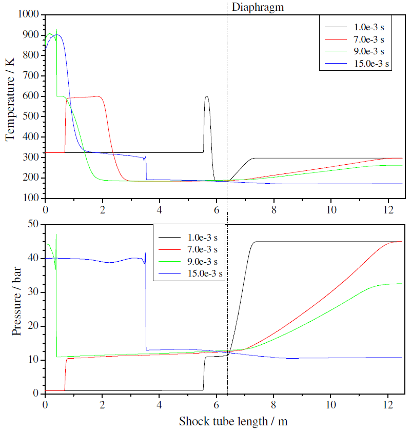
Figure 5. Predicted (a) temperature and (b) pressure distributions along the shock tube for different elapsed times using κ-ε
4.2.1. Incident shock wave
Figure 6 presents the contour plots for (a) Mach number, (b) pressure and (c) turbulence intensity predicted by the κ-ε turbulence model at 1×10^(-3) s after bursting of the diaphragm. In Figure 6(a), the incident shock wave position is seen at 0.86 m from the position of the diaphragm. The position of the expansion fan is visible in the pressure contours in Figure 6(b). The contact surface is seen at Figure 6(c) at ~0.75 m from the diaphragm. From Figure 6(c), we note that the region behind the contact surface presents higher turbulence levels. These higher turbulence levels affect the flow behind the contact front, but not in front of the incident and behind the reflected waves. Turbulence levels in front of the incident wave are virtually zero. This explains why the velocity of the incident wave is unaffected by the choice of turbulence model, as long as the model is consistent for low turbulence (i.e., tends to the formulation without turbulence model for low Reynolds). Comparing the values of the conditions behind incident shock from Table 3, with the mean values of Figure 6 for Mach Number and (b) pressure, one can see that the CFD simulation underestimates the Mach number by about ~50%, the temperature behind the incident shock is in good agreement with the 1D-solution and the pressure is overestimated in about ~40%.
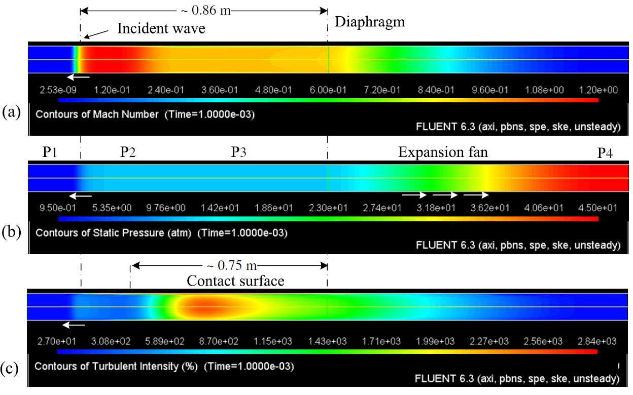
Figure 6. Flow at 1×10^(-3) s predicted using the κ-ε turbulence model
4.2.2. Reflected shock wave
Figure 7 presents the numerical results at time 8.5×10^(-3) s predicted with the Reynolds Stress Model (RSM) for (a) Temperature, (b) Mass Fraction of Ethanol and (c) Turbulent Intensity. At this ellapsed time, the reflected shock wave and the contact surface are moving in opposing directions. The contours of temperature, Figure 7 (a), show that the reflected shock wave is about ~0.24 m from the shock tube end wall. The contact surface, Figure 7(b), is about ~1.12 m from the end wall and the high turbulence levels now are behind the reflected shock wave and close to the wall, Figure 7(c). Figure 7(b) shows the evolution of the contact surface profile. The contact surface starts like a plane, but soon it acquires a parabolic profile, as a result of the boundary layer created behind the shock wave. Comparing the values of the conditions behind reflected shock from Table 3, with the mean values of temperature from Figure 7(a) one can see that temperature behind the incident shock agrees with the 1D-solution.
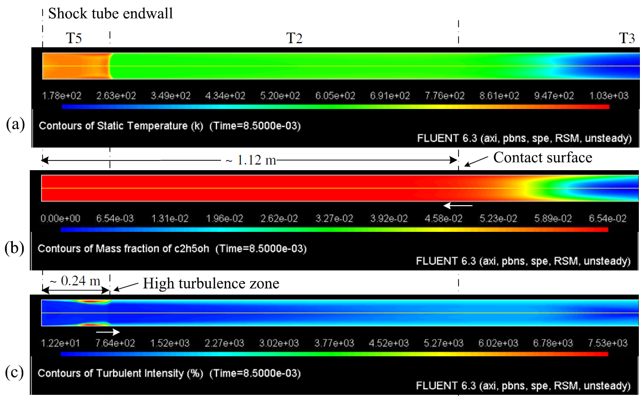
Figure 7. Flow at 8.5×10^(-3) s predicted using the RSM turbulence model
5. Conclusions
This work is an attempt to analyze by numerical simulation the propagating shock wave in a shock tube as an aid for the design and operation of shock tubes for chemical kinetic studies. Here, the structure of the compressible flow in a shock tube experiment was simulated for the conditions of the high-pressure shock-tube at the University of Duisburg-Essen for a stoichiometric mixture of ethanol and air. A structured mesh with 0.5 mm of spatial resolution was used. The time discretization was fixed in 1×10^(-5) s. Three turbulence models available in FLUENT, the standard κ-ε, the κ-ω and the Reynolds-Stress models, and a simulation without turbulence model model were tested.
The results from all CFD models compared qualitatively well to one-dimensional predictions of the shock wave properties using the SHOCK package of CHEMKIN. However, while incident shock wave speed was well predited when compared to the measurement, all models overestimated the refleted shock wave speed when compared to SHOCK in about 10-30%. The RANS models captured the effect of the boundary layer growth behind the incident wave. Higher turbulence levels were located behind the contact surface in the core flow and behind the reflected shock wave near the walls. While temperatures behind incident and refleted shock waves are well predicted, all models failed to correctly predict the pressures, yielding similar errors of about 30-40%. It is not clear so far whether a more refined grid would capture the pressure increase, or if this would not be possible using a RANS model. Simulations using a more refined mesh and comparison to LES models are necessary to further assess the possibilities in modeling shock tubes.
Acknowledgements
The authors gratefully acknowledge the CNPq – Brazil, DAAD and DGF – Germany, for the support given in the development of this work, and Mr. M. Longo for setting up the computer network for parallel processing.
References
- Al-Falahi A., Yuso® M.Z., Yusaf T., (2007). 16th Australasian Fluid Mechanics Conference. Crown Plaza, Gold Coast, Australia.
- Bird R.B., J.O. Hirschfelder., C.F. Curtis., (1954). Molecular Theory of Gases and Liquids. JOHN WILEY & SONS, INC. USA.
- Cancino L.R., Oliveira A.A.M, Fikri M., Schulz C. (2009). ISSW-27, paper 30074.
- Edwards, J.R. (2008). Progress in Aerospace Sciences 44, 447465.
- Fluent 6.3 Documentation (2006). FLUENT INC., Copyright 2006, FLUENT INC. Available at: www.fluentusers.com
- Gibson M.M. and Launder B.E. (1978). J. Fluid Mech., 86:491-511, 1978.
- Kee R.J , F.M. Rupley, J.A. Miller, M.E. Coltrin, et al., (2000). CHEMKIN Collection, Release 3.7.1, Reaction Design, Inc., San Diego, CA.
- Knight, D., Yana H., Panaras A.G. and Zheltovodovc A. (2003). Progress in Aerospace Sciences 39, 121184.
- Launder B.E. (1989) Inter. J. Heat Fluid Flow, 10(4):282-300.
- Launder B.E. and Spalding D. B. (1972). Lectures in Mathematical Models of Turbulence. Academic Press, London, England.
- Launder B.E., G.J. Reece, and W. Rodi. (1975) J. Fluid Mech., 68(3):537-566
- Mirels, H. (1963). Test Time in Low-Pressure Shock Tubes., THE PHYSICS OF FLUIDS., Volume 6, Number 9.
- Mundt C., Boyce R., Jacobs J., Hannemann K. (2007). Aerospace Science and Technology 11, 100109.
- Pope. S.B. (2000). Turbulent Flows. Cambridge University Press. UK
- Rudinger, G. (1961). The Physics of Fluids., Volume 4, Number 12.
- Saad M.A., (1993). Compressible Fluid Flow. 2nd Ed. Prentice Hall. USA
- Sod G.A. (1978). J. Comput. Phys. 27 p. 1-31.
- Tsuchida J., Fujisawa T., Yagawa G. (2006) Comput. Methods Appl. Mech. Engrg. 195, 1896-1910.
- Wilcox D.C. (1998). DCW Industries, Inc., La Cañada, California
- Zel’dovich Ya.B., Raizer Yu.P., Hayes W.D., Probstein R.F. (1966). Physics of ShockWaves and High-Temperature Hydrodynamic Phenomena. Volume I. ACADEMIC PRESS, New York and London.
- Zel’dovich Ya.B., Raizer Yu.P., Hayes W.D., Probstein R.F. (1966). Physics of ShockWaves and High-Temperature Hydrodynamic Phenomena. Volume II. ACADEMIC PRESS, New York and London.
Note: This work was published in the 27th International Symposium on Shock Waves – 19..24 July-2009, St. Petersburg
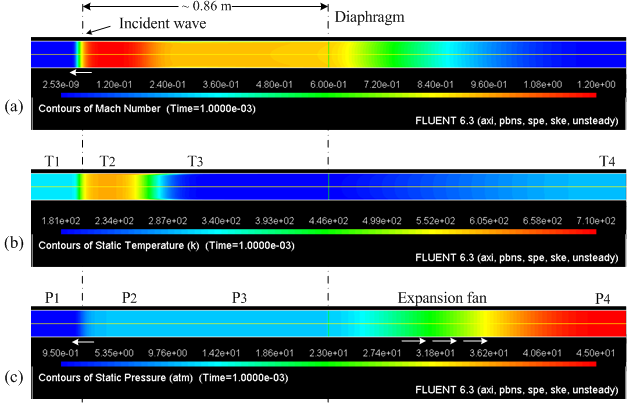
Figure 6(a). Flow at 1×10^(-3) s predicted using the κ-ε turbulence model (additional data-postprocessing)
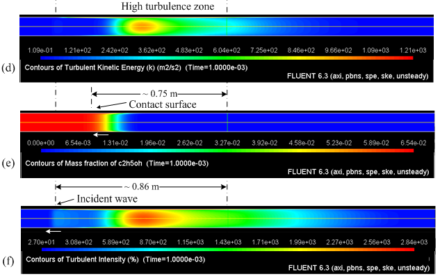
Figure 6(b). Flow at 1×10^(-3) s predicted using the κ-ε turbulence model (additional data-postprocessing)
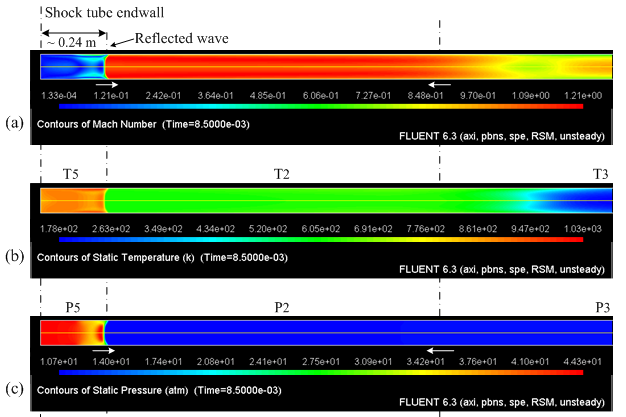
Figure 7(a). Flow at 8.5×10^(-3) s predicted using the RSM turbulence model (additional data-postprocessing)
Figure 7(b). Flow at 8.5×10^(-3) s predicted using the RSM turbulence model (additional data-postprocessing)