

Interação térmica chama/estrutura em queimadores


A numerical study of the heat recirculation across the flame-solid interface in stabilised flames of propane and n-butane
Leonel Rincon Cancino, Dr. Eng., leonel@labcet.ufsc.br
Amir Antônio Martins Oliveira, Ph.D., amir.oliveira@gmail.com
Combustion and Thermal Systems Engineering Laboratory . LabCET
Mechanical Engineering Department
Federal University of Santa Catarina
Brazil.
Abstract. In this work, a numerical study of the flame-solid interaction in propane and n-butane supported flames is presented. The fuel-air partially premixed flames (stoichiometric ratio of 0.6) are attached to an orifice in the top side of a circular stainless-steel plate. The flow ranges from laminar to slightly turbulent, which is typical of domestic applications. The analysis employs a turbulence model (k-e model) and a global single-step chemical reaction mechanism for the gas phase and conduction heat transfer along the steel plate. The geometry is axisymmetric and the equations are solved using the CFD solver FLUENT. Two methods for the chemistry-turbulence interaction are tested and the results are compared. The coupling of the solid and gas phases render the solution expensive in terms of computational time. This is a serious drawback for the use of more complex chemical reaction mechanisms. The results evidence the role of the heat recirculation along the steel plate to the unburned gas mixture in the flame temperature and flame speed. Results are presented for both fuels, evidencing the effects of the ratio between chemical kinetic characteristic time scale and convection-conduction corresponding time scales. Surface heat transfer convection coefficients are also presented.
INTRODUCTION
The maximum value or final temperature in a combustion process depends of the initial thermal level of the reactants. In practical applications, have a heat flux of the flame to metallic support. The metallic support is heating by the flame in the combustion-side and is cooled by the fresh mixture in the internal side. This flux allows a preheating in the fresh mixture before to combustion process. In numerical simulations this preheating process is difficult to capture and to evaluating. Figure 1 shows this process.

Figure 1. Heat recirculation
In combustion process, the thermal level attached by the metallic support is an important parameter for the flame stabilization.
SIMULATION AND COMPUTATIONAL DOMAIN
Geometry
In this work, a simplified geometry was employed. Is analyzed a standalone flame formed in the superior side of a circular plate of steel. The thickness of the plate is e = 0.6 mm, and the diameter is D = 70 mm, the Figure 2 shows the principal characteristics.
Computational mesh
The 3D geometry of the physical model is approached to a 2D axial-symmetric geometry. The axial-symmetric characteristic allows in a 2D solution, capture the full 3D aspects of the process in question, reducing the computational effort in the problem solution. Hybrid structured/unstructured mesh was employed in this simulations and a boundary layer was imposed in all surfaces of the solid shape that is in contact with the fluid domain. Figure 2 show the geometry and the mesh.
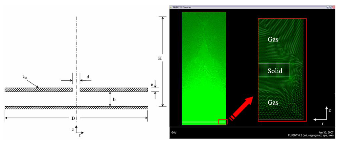
Figure 2. Geometry and computational mesh
The fluid and solid phase are thermally coupled; this fact allows the heat recirculation in the two phases. A boundary layer was created in the fluid phase in contact with the solid support. This boundary layer has a great refinement in the normal direction of the solid phase (high temperature gradients) attempt to capture the heat recirculation of an adequate form.
Numerical simulation
In a real combustion process, several hundred of chemical reactions occur simultaneously (Cancino 2004, Cancino and Oliveira 2004, 2005, 2005b) and several hundreds of chemical species are involved. For the methane – air reacting system, the scientific community has adopted the GRIMech 3.0 reaction mechanisms as a best detailed kinetic model, this mechanism have 354 chemical reaction and 53 chemical species. A detailed kinetic model for the i-Octane oxidation can be composed by a set of around of 4000 chemical reactions (Curran, 2002).
Solvers of CFD programs have a limit in function of the actual computational resources (Westbrook, 2005), the solver need processing the set of equations for conservation of momentum, turbulence, radiation and more one equation by each chemical species considered in the combustion process. If in the combustion process are considered more of ten chemical species, the set of equations for the chemical species conservation is more complicated, computationally, that the rest of the problem. This complication can rise in function of the turbulence-chemical kinetics interaction model.
In this work, the combustion process is approached by a global kinetic model with one step – chemical reaction. Two models for the turbulence-chemistry interaction process are used, the Eddy-Dissipation Model (ED) and the Eddy-Dissipation Concept (EDC). The computational time is expensive in function of the thermal solid-fluid couplement. In these simulations, the two phases are coupled thermally, a heat flux is induced by the flame hot zone to the plate, and the plate by heat conduction is heating the fresh mixture of gas unburned. The solid phase has a great thermal inertia, in the gas phase a change in the thermal level is absorbed rapidly by the solver. These differences in the thermal inertias of the two phases render a slow convergence process.
Two fuels are considered in this work, butane and propane and was used the FLUENT CFD commercial program for the numerical simulation. A total of four simulations were made in this work:
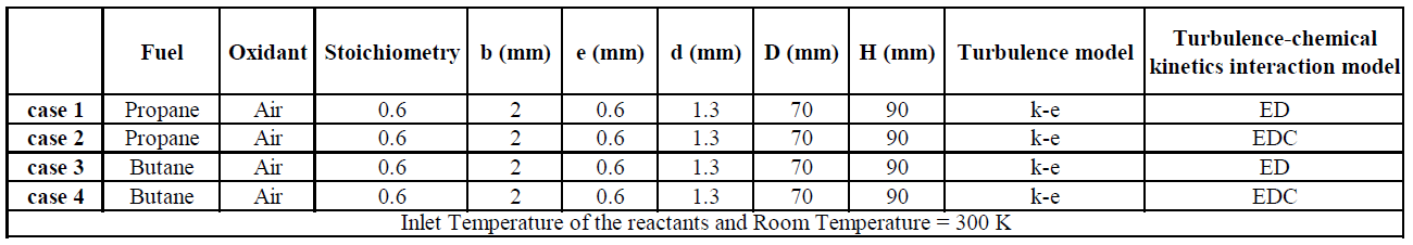
Table 1. Cases considered in this work for simulation
Combustion models, Turbulence model and Turbulence-chemistry interaction
Several methodologies are used for the numerical representation of a combustion process. The selection of the combustion model is in function of the target to be captured in the simulation. In this work, the target was to capture the effect of the heat recirculation, in the solid support to the fresh mixture, in the final flame temperature and configuration. In combustion modeling, have been proposed different methodologies to manage the problem of the turbulence-chemistry interaction, these approaches can be grouped in three great sets (Stefanidis, 2006): a) statistical approaches, b) flamelet models, and c) reaction rate – turbulence levels direct relations models.
In the first set, is common to use Provability Density Functions PDF’s to determine the mean values of scalar or velocity scalar, Zhang 2005, has reported this methodology like a powerful tool for the numerical simulation of combustion process in HCCI engine combustion. The second set is based in the geometrical analysis of the flame; all reactions are considered to be sufficiently fast so that the length scale of the reaction zone is smaller than the Kolmogorov length scale. In this case, the flame can be considered as an ensemble of very thin, isotropic, one-dimensional laminar flame structures (flamelets). The third set of turbulence–chemistry interaction models consists of models that relate the effective reaction rates to turbulent mixing levels. In this work, we have taken two models for the comparison, the Eddy Dissipation Model and the Eddy Dissipation Concept; these models are classified in the third set of approaches above mentioned.
In this work, the gas phase is composed by two zones. This division of the gas phase was to define the reaction zone. The gas zone down of the plate is assumed without chemical reaction. The gas zone upper of the solid plate is assumed with chemical reaction. The two gas phases are coupled thermally in the numerical interface, of this form is included the effect of the heat flux between gas phases by diffusion. Was used the Full-multicomponent Diffusion Option in the Solver´s Options of the CFD.
Turbulence model
In this work, we use the well-know κ – ε turbulence model. This model assume that the flow is fully turbulent but, when the model identify a laminar regimen region, the model capture this effect and it return a laminar solution for the fluid flow. This model will go to provide the two principal parameters for the turbulence-chemistry approach adopted in this work, the Turbulence Kinetic Energy (κ) and the Dissipation Rate of Turbulence Kinetic Energy ( ε ). Several authors has used the κ – ε turbulence model in simulation of combustion process of hydrocarbons, obtaining good results, (Gu 2005, Cancino and Oliveira 2006, Heynderickx 2005), Wilcox 1994 shows the whole methodology and applications for the κ – ε turbulence model.
Eddy Dissipation Model
This model is recommended for flows with a high turbulence. For many flows with this characteristic, the overall rate of reaction is controlled by turbulent mixing. In this model, the Arrhenius rate is not used to determine the production/destruction of chemical species, instead, other formulation is proposed to determine the species source term in the species conservation equation.
Eddy Dissipation Concept
In this model, is assumed that the chemical reaction occur in the small turbulent structures named “fine scales”. This model is an extension of the ED model to include the effect of the detailed chemical mechanisms in turbulent flows. The traditional species source term in the species conservation equation is changed too, and a new term is proposed. This new term involve length and time scales defined for the chemical reaction, inside of this “fine scales”, is assumed that the combustion process occur at the same form that in a Perfect Stirred Reactor – PSR, no spatial variation of chemical species is considered and the combustion proceed in a homogeneous ambient, is applied the Arrhenius model to calculate the local production/destruction of species, after, the values of the concentrations are used to obtain the mean values of the concentration outside of the “fine scales”.
RESULTS
In a simulation process, is very rich the quantity of information that can be extracted of the solution. In this work, the focus of analysis was the heat recirculation of a global form. The results presented allow temperature distribution in all phases of the computational domain, surface heat transfer coefficients in the walls of the plate (solid support), and velocity fields in the gas phase.
Temperature Analysis
The Figure 3 shows the temperature distribution in the solid phase (plate) of the four cases simulated in this work.
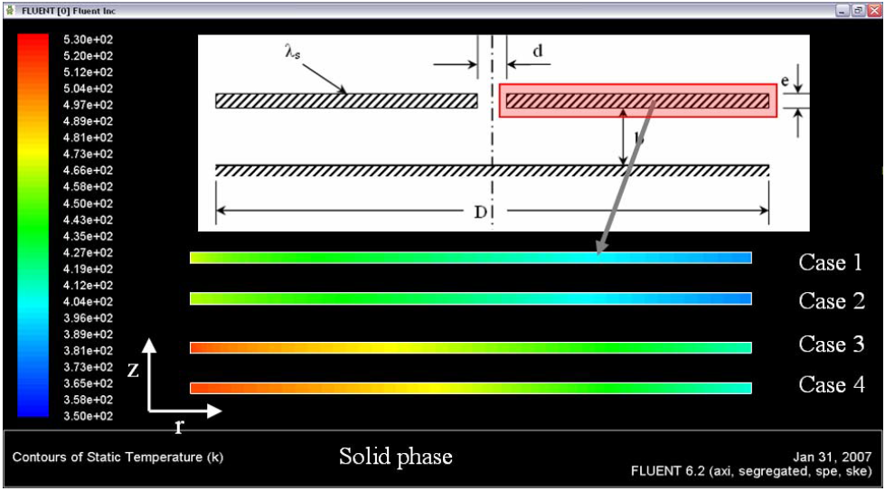
Figure 3. Temperature distributions in the solid phase – plate
Figure 3 shows the radial and axial temperature in the solid support. The combustion process takes place in the upper-right side of the plate. The thermal level attached by the solid phase in the combustion process of butane is bigger to thermal level attached by the propane. Figure 4 shows the superficial temperature in the internal and external walls of the solid support for the four cases.
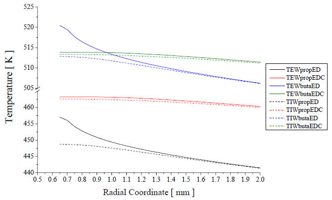
Figure 4. Superficial temperature distributions in the internal and external walls of the plate
The Figure 4 was plotted for the first 2 mm of the radial length of the plate shows that the major temperature difference between the internal and external walls is in the first millimeter of the plate in direction radial, starting in the hole, for the Eddy Dissipation Model (ED) for the turbulence-chemistry interaction. After of the 2 mm, the values of the internal and external wall temperature are the same or differ in a small amount.
This fact can indicate that the major heat transfer process of the burned gas phase to the fresh mixture occur in the first millimeter in the radial direction. This fact is a consequence of the radial distribution of the fluid field, for this geometry, the flow is accelerated in the nearness of the hole in the inferior side of the plate, when the mixture has not burned yet.
High values of velocity yield a high value of the local surface heat transfer coefficient, increasing the convection heat transfer rate. In the edge of the hole, the ED model forecast high values for the surface heat transfer coefficient, 4215 W/m2 K for propane and 2682 W/m2 K for butane. For the Eddy Dissipation Concept (EDC), the forecast was of minor values, 142 W/m2 K and 82 W/m2 K, respectively.
The Figure 5 shows the heat recirculation across of the flame-solid interface. The heat flux direction is observed numerically by the sign of the surface heat transfer coefficient. In the external wall of the plate, there are changes in sign of the surface heat transfer coefficient (SHTC), pointed to two direction of the heat flux. In the first millimeters of the superior wall, there are high values of the SHTC indicates that a great quantity of heat is incoming to solid phase and leaving the gas phase (flame source).
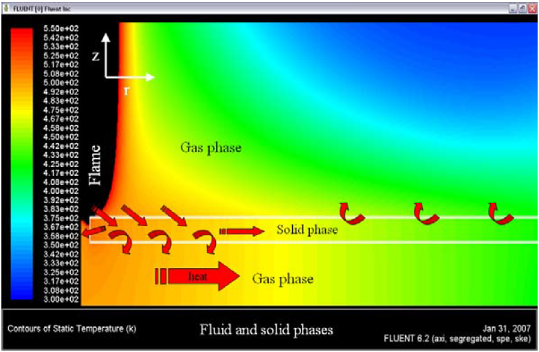
Figure 5. Heat recirculation in the solid and fluid phases
The Figure 6 shows the total surface heat flux for two cases. The ED model forecast high values of SHTC, this fact increase the heat transfer process in the first millimeters of the plate around of the central hole. The ED model is recommended for flows with a high turbulence intensities, in this case, the edge of the hole is a geometrical configuration that yield a great production of Turbulence kinetic energy, this fact is reflected in the reaction rate described in the equation (1) or (2), rising its value and overestimating (in this case) the thermal and fluid-dynamic fields.
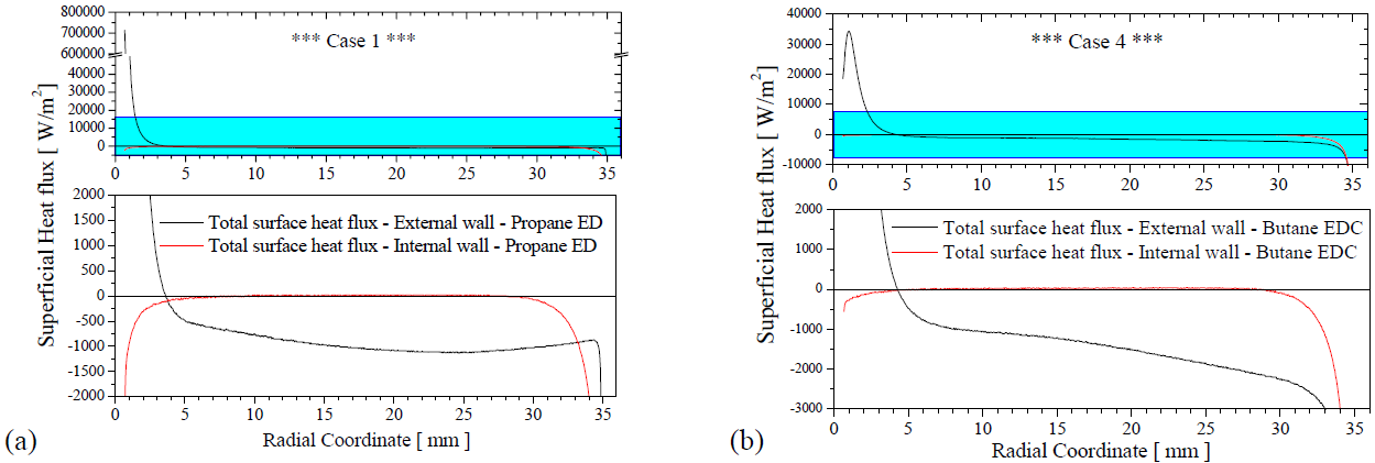
Figure 6. Total surface heat flux in the external and internal walls of the plate (solid domain)
Temperature field for all cases simulated in this work, are showed in the Figure 7. In this figure, can be observed the dissimilarity in the flame position, foresee for the two turbulence-chemistry interaction methods used in the simulations. The ED model indicates that the flame is located and “prey” to the edge of the hole, in cases one and three. This fact demand the predict of high values of SHTC and this overestimate the surface heat flux in the first millimeters of the plate, for the ED model, a surface heat flux of ~ 700000 W/m2 is calculated by the CFD solver (see Figure 6 (a)) this is a consequence of the high values of temperature, velocities and turbulence kinetic energy calculates in this location (see Figure 7 , Figure 8 and Figure 9).
The EDC model calculate a surface heat flux of ~ 20000 W/m2 in the same position, and a surface heat flux of ~ 40000 W/m2 in the region that the flame is more close to plate (see Figure 6 (b)). The zone of penetration of heat of the flame to the plate is, in dimension, a little bigger in the EDC model when compared with the ED model (see Figure 6, positive surface heat flux), this heat flux is conducted by the solid plate and it is leaving the plate by convection superficial in the external and internal faces of the plate (see Figure 5)
Fluid-dynamic Analysis
The Figure 8 shows the velocity field in all simulations. The ED model predicts major velocity values for the flame speed, when compared with the values predicted for the EDC model. The ED model is not influenced by the global one step – kinetic model, the ED model take the values of ê and e of the turbulence model and via equation (1) or (2), it calculates the species concentrations, this concentrations are influencing in the energy equation in the mass diffusion term.
In the EDC model, the solution is influenced by the global one-step kinetic model. It use the Arrhenius parameters (imposed for the model) to calculate the formation/destruction of species, of indirect form, the results are influenced by the parameters of the kinetic model (pre-exponential factor and Activation energy principally) The solution of the set of conservation equations by the CFD solver is coupled, any alteration in a term in some conservation equation is transported to the whole set of equations, the flaws can be propagate and end up with the alteration of the result in all variables transported/analyzed in the problem.
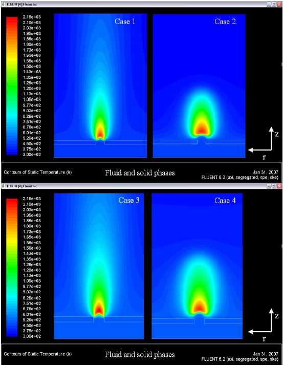
Figure 7. Temperature distributions in the solid and fluid phases
In this case, the ED model is overestimating the velocities; values of flame speed of ~ 3.0 m/s are not reported in the literature for the reacting systems propane-air and butane-air, in reacting flows with a Reynolds number of ~ 2.5. The prevision of velocities by the EDC model is more realistic, values of flame speed of ~ 0.8 m/s with the same conditions of Reynolds number ~ 2.5 in the hole. Figure 9 shows the fields of turbulence kinetic energy. In this figure can be identified the production of k in the edges of the hole.
For the model ED, this production of ê imposes the combustion process just in this location (the edge of the hole). In the results for the EDC model, exists production of ê in the edges too, but the flame is stabilized a little above of the hole, in other words, the geometrical influence of the plate in the production of ê in the flow field about the edge of the hole is not influencing for the flame stabilization, numerically spoken.
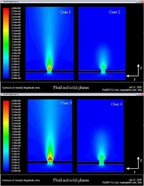
Figure 8. Velocity fields (gas phase)
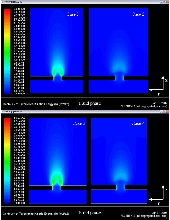
Figure 9. Velocity fields (gas phase)
The Figure 10 shows the temperature and velocity distribution in the first millimeters of the axis in the computational domain, for the four cases. Adopting the rise of temperature with an indicative for the flame position, the model EDC indicates that the flame is located a little more far of the hole, when it is compared with the ED model.
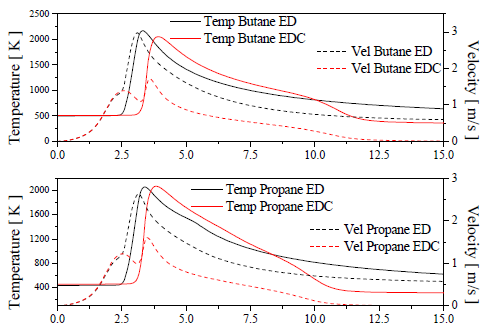
Figure 10. Temperature and velocity distribution in the central line of the computational domain
The Figure 11 shows several profiles of temperature and velocity for the simulation case 2, propane-air with the EDC model for the turbulence-chemistry interaction. In z = 2.6 mm is located the exit of the hole, the Figure 11 shows that the reactant mixture is heating nearest to edge of the hole, this is a effect of the heat recirculation. This recirculation yields an increment in the temperature of the reactants of ~ 161 °C, the reactants are inlet to computational domain at 300 ° C and before of the flame, it are at 461 °C in the center of the exit hole without combustion yet.
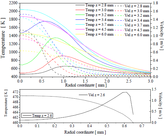
Figure 11. Temperature and velocity profiles, case 2, Propane-air with EDC model
CONCLUSIONS
In this work, a numerical study of the flame-solid interaction in propane and n-butane supported flames is presented. The analysis employs a turbulence model (ê-å model) and a global single-step chemical reaction mechanism for the gas phase and conduction heat transfer along the steel plate. Two methods for the chemistry-turbulence interaction are tested and the results are compared. The coupling of the solid and gas phases render the solution expensive in terms of computational time.. The results evidence the role of the heat recirculation along the steel plate to the unburned gas mixture in the flame temperature and flame speed.
About of the turbulence-chemistry interaction methods:
- The ED model is overestimating the velocities; values of flame speed of ~ 3.0 m/s are not reported in the literature for the reacting systems propane-air and butane-air, in reacting flows with a Reynolds number of ~ 2.5.
- The prevision of velocities by the EDC model is more realistic, values of flame speed of ~ 0.8 m/s with the same conditions of Reynolds number ~ 2.5 in the hole.
- For the model ED, the production of ê imposes the combustion process just in this location (the edge of the hole).
- In the results for the EDC model, exists production of ê in the edges too, but the flame is stabilized a little above of the hole, in other words, the geometrical influence of the plate in the production of ê in the flow field about the edge of the hole is not influencing for the flame stabilization, numerically spoken.
- The EDC model shows a best performance for this type of simulations.
About of the heat recirculation in the plate:
- The major temperature difference between the internal and external walls in the solid support is in the first millimeter in direction radial, starting in the hole, for the Eddy Dissipation Model (ED) for the turbulence-chemistry interaction. After of the 2 mm, the values of the internal and external wall temperature are the same or differ in a small amount.
- This fact can indicate that the major heat transfer process of the burned gas phase to the fresh mixture occur in the first millimeter in the radial direction. This fact is a consequence of the radial distribution of the fluid field, for this geometry, the flow is accelerated in the nearness of the hole in the inferior side of the plate, when the mixture has not burned yet.
- High values of velocity yield a high value of the local surface heat transfer coefficient, racing the convection heat transfer rate. In the edge of the hole, the ED model forecast high values for the surface heat transfer coefficient, 4215 W/m2 K for propane and 2682 W/m2 K for butane. For the Eddy Dissipation Concept (EDC), the forecast was of minor values, 142 W/m2 K and 82 W/m2 K, respectively.
- The heat flux direction is observed numerically by the sign of the surface heat transfer coefficient. In the external wall of the plate, there are changes in sign of the surface heat transfer coefficient (SHTC), pointed to two direction of the heat flux. In the first millimeters of the superior wall, there are high values of the SHTC indicates that a great quantity of heat is incoming to solid phase and leaving the gas phase (flame source).
- The heat recirculation, for the EDC model in the propane-air system (case 2), yields an increment in the temperature of the reactants of ~ 161 °C, the reactants are inlet to computational domain at 300 ° C and before of the flame, it are at 461 °C in the center of the exit hole without combustion yet. A similar performance was observed for the system butane-air (case 4).
About of simulation process:
- The simulation of a combustion process including the couplement of the gas and solid phases is computationally expensive. The computational time for each simulation in this work was 25 days in full time, employing a PC Desktop Pentium IV, 3.4 GHz, 4 GB RAM memory (Random Access Memory) with local parallel process (two process).
- The difference in the computational time between the two turbulence-chemistry interaction is small, but, computationally is more hard to processing the EDC model in the starting process (firsts 10 days…), when is imposed one step-solution of the chemistry for each step-solution of the fluid-dynamic.
- Inlet Temperature of the reactants and Room Temperature = 300 K
ACKNOWLEDGEMENTS
The authors gratefully acknowledge the Graduate Program in Mechanical Engineering at UFSC – POSMEC and the CNPq, for the support given in the development of this work.
REFERENCES
- Cancino, L. R. and Oliveira, A. A. M., 2005 b, “Analysis of the thermal ignition and induction time of premixed ethanol and air combustion”. Proceedings of the 18th International Congress of Mechanical Engineering. COBEM 2005. Brazil.
- Cancino, L. R. and Oliveira, A. A. M., 2004, “Análise de equilibrio químico, cinética química da ignição térmica e propagação de chama plana laminar de misturas de hidrocarbonetos leves com ar”. Proceedings of the ENCIT 2004, Rio de Janeiro, Oct. 2004, 11 pp.
- Wilcox, D. C. “Turbulence modeling for CFD” DCW Industries, INC. La Cañada, California. 1994.
- Cancino, L. R. and Oliveira, A. A. M., “Influência da insaturação do carbono sobre o equilíbrio químico e ignição térmica de hidrocarbonetos alifáticos em ar”. Proceedings of the X Latinamerican Congress of Heat and Mass Transfer. 2005, Caracas, Venezuela.
- Cancino, L. R., 2004, “Análise de equilíbrio químico, cinética química da ignição térmica e propagação de chama plana laminar de misturas de hidrocarbonetos leves com ar”. Dissertation of Master degree at the Federal University of Santa Catarina, 2004, in Portuguese, 245 pp
- Curran, H. J., Gaffuri, P., Pitz, W. J. and Westbrook, C. K., “A Comprehensive Modeling Study of iso-Octane Oxidation”, Lawrence Livermore National Laboratory, Livermore, CA 94551, USA, 2002,
- GRIMech Gas Research Institute. Disponível em: < http://www.me.berkeley.edu/gri_mech/ > GRIMech 3.0 (2000).
- Westbrook, C, K., Mizobuchi, Y., Poinsot, T, J., Smith, S., Warnatz, J. “Computational Combustion.” Proceedings of the Combustion Institute. 30 (2005). 125-157.
- Stefanidis, G.D., Merci, B., Heynderickx, G.J., Marin G.B. “CFD simulations of steam cracking furnaces using detailed combustion mechanisms”, Computers and Chemical Engineering 30 (2006) 635–649.
- Zhang, Y.Z., Kung, E.H., Haworth, D.C. “A PDF method for multidimensional modeling of HCCI engine combustion: effects of turbulence/chemistry interactions on ignition timing and emissions” Proceedings of the Combustion Institute 30 (2005) 2763–2771.
- Gu, S., Kamnis, S. “Numerical modelling of propane combustion in a high velocity oxygen–fuel thermal spray gun” Chemical Engineering and Processing 45 (2006) 246–253.
- Cancino, L. R. and Oliveira, A. A. M., 2006, “ANÁLISIS NUMÉRICO DEL PROCESO DE COMBUSTIÓN EN UN QUEMADOR TIPO FLAUTA DE APLICACIÓN DOMESTICA”. Tercer Congreso Internacional de Ingeniería Mecánica y Primero de Ingeniería Mecatrónica. CIMM 2006. Bogotá – Colombia.
- Heynderickx, G.J., Stefanidis, G.D., Merci, B., Marin, G.B. “CFD simulations of steam cracking furnaces using detailed combustion mechanisms” Computers and Chemical Engineering 30 (2006) 635–649.
- Fluent 6.2 Documentation. Fluent Inc.
Note: This work was published in the 19th International Congress of Mechanical Engineering, November 5-9, 2007, Brasília, DF. Proceedings of COBEM 2007 Copyright © 2007 by ABCM